The Coefficient of Determination and Adjusted R-Squared
I once had the opportunity to listen to a colleague present some modeling results. While discussing their model selection procedure, my colleague compared different models using the R-squared statistic - also known as the coefficient of determination. This often cited statistic can tell us how well a model fits a given dataset. It is interpreted as the percentage of variance in the dataset that is explained by the model. A handy tool, right? However, it comes with some caveats as we will see.
The reason I was inspired to write this post is that, during the aforementioned engagement, my colleague stated that they chose to include a few different covariates because “the R-squared value increased when they were added to the model.” On its face that seems like a good decision. If the percentage of variance explained by the model increases with new covariates, then the model is doing a better job at explaining the relationships between covariates and the response variable, right? Unfortunately, it isn’t that simple. Let’s look at an example in code:
For this blog post I’m using the following libraries:
import matplotlib.pyplot as plt
import numpy as np
from sklearn.linear_model import LinearRegression
from sklearn.metrics import r2_score
Next we will define a target function that we want to approximate and simulate some data. Note that the first term in our function is squared. In the real world very few functions are truly linear in the predictors, but in many cases we can approximate non-linear functions with linear regression.
def target_function(x1, x2, x3):
    return x1 ** 2 - 5 * x2 + (1/3) * x3

rng = np.random.default_rng(seed=42)

n = 100

x1_data = rng.uniform(1, 3, n)
x2_data = rng.uniform(0, 1, n)
x3_data = rng.uniform(1, 10, n)

noise = rng.normal(size=n)

y = target_function(x1_data, x2_data, x3_data) + noise
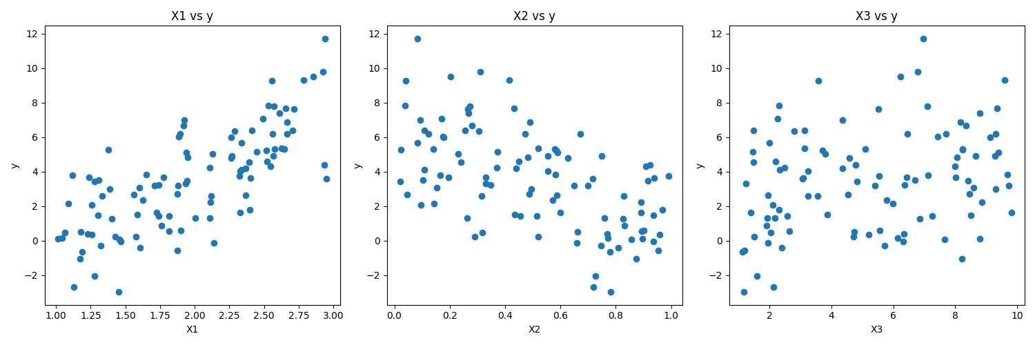
This is what the data looks like in scatter plots:

Now let’s fit a model and calculate the R-squared value.
X = np.c_[x1_data, x2_data, x3_data]

model = LinearRegression()
model.fit(X, y)

preds = model.predict(X)
r2 = r2_score(y, preds)
print(f"R^2 Score: {r2}")

>>> R^2 Score: 0.8728
The R-squared value produced by this code is about \(0.8728\). That means that our model is able to account for roughly \(87.28\%\) of the variance in the response variable. Because we defined the function ourselves (that is to say, the process by which our response variable is generated), we can say that this is a truthful representation of the quality of our model. But what happens if we were include an entirely unrelated covariate in our model? Intuitively, the R-squared value should not increase because we can’t explain variation in our response variable using an entirely unrelated predictor variable.
x4_data = rng.normal(size=n)
X_prime = np.c_[X, x4_data]

model = LinearRegression()
model.fit(X_prime, y)

preds = model.predict(X_prime)
r2 = r2_score(y, preds)
print(f"R^2 Score: {r2}")

>>> R^2 Score: 0.8748
The coefficient of determination has increased. In fact, we will see an increase - or at least no decrease - with every new covariate no matter the relationship with the response variable. Surprisingly, this increase in R-squared is not due to our new covariate providing any real insight into the response variable. Rather, it is a mathematical artifact of how R-squared is calculated. The addition of any new variable, regardless of its actual relevance, can capture some additional variance by chance. This leads to an increase in the R-squared value, even though the added variable might be completely unrelated to the response variable. This phenomenon is known as “spurious correlation,” where the model appears to improve simply because it has more variables.
We still want to compare models with different covariates. For this we can turn to the adjusted R-squared calculation which penalizes R-squared based on the number of covariates in the model. Here is a python function calculating adjusted R-squared.
def adjusted_r2_score(r2, n, p):
    return 1 - (1 - r2) * ( (n - 1) / (n - p - 1) )
Now let’s add several covariates one-by-one and watch what happens to the R-squared and adjusted R-squared values over time. Here is the code:
def get_new_covariate(Xdat, number_generator):
    dsize = Xdat.shape[0]

    new_mean = number_generator.normal()
    new_std = number_generator.gamma(shape=1.0)

    x_new = number_generator.normal(new_mean, new_std, size=dsize)
    return np.c_[Xdat, x_new]

r2_scores = []
adj_r2_scores = []

for i in range(5):

    X = get_new_covariate(X, rng)
    n_covariates = X.shape[1]

    model = LinearRegression()
    model.fit(X, y)

    preds = model.predict(X)

    r2 = r2_score(y, preds)
    adj_r2 = adjusted_r2_score(r2, y.size, n_covariates)

    r2_scores.append(r2)
    adj_r2_scores.append(adj_r2)
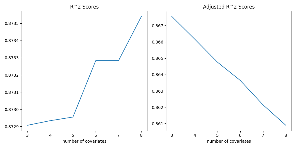
And here are plots that show the change in R-squared and adjusted R-squared values:

When we run this code we see that, while R-squared is monotonically increasing (or at least staying the same), the adjusted R-squared is either lower or does not increase as much as the original R-squared upon adding an irrelevant variable. This serves as a reminder that while R-squared can be a useful metric, it should be interpreted with care, especially in models with a large number of covariates. The adjusted R-squared provides a more realistic assessment of model performance by accounting for the complexity of the model.
The journey through R-squared and its adjusted counterpart in this post illuminates a fundamental principle in statistical modeling: simplicity and relevance are key. While R-squared can give an initial impression of a model’s explanatory power, it’s crucial to look beyond the surface. The inclusion of unnecessary covariates, as demonstrated, can artificially inflate R-squared, leading us down a misleading path of perceived accuracy. Adjusted R-squared offers a more nuanced and honest evaluation, guiding us towards models that are not just statistically sound but also meaningful and practical. As data scientists and statisticians, our aim should always be to strike a balance between model complexity and explanatory power, ensuring that our models capture the essence of the data without adding needless complexity. In the realm of data modeling, sometimes less is more.